Computer codes
To use these codes, download the archived compressed file
filename.tar.gz, open and decompress the file by running the
commands (on unix-based systems): tar xvf filename.tar.gz; gunzip
filemane.tar. You can then run the script main.m in matlab.
For each code, I propose a few tasks to experiment the properties of
the flows. Feel free to edit these scripts, implement loops to test many parameters,
compare your results to what is written in books and articles...
For bugs, comments and questions,
contact me.
Spatial/temporal stability analysis of the mixing layer
Description:
For parallel flows, one distinguish the spatial and the temporal stability analyses, whether the flow solution is allowed to grow exponentially in space or in time. This code computes the eigenmodes for the two situations for a mixing layer. The base flow profile is an hyperbolic tangent, and the system is discretized using Chebychev collocation.
From the spectrum, one sees clearly two families of modes: one with support on the upper stream (the fast one), and one with support in the lower stream. For these two families, the eigenmodes are advected with the flow. These eigenmodes are increasingly oscillating as they are more damped, and do not tend to zero away from the shear region: these belong to the continuous spectrum. There is as well one unstable eigenmode (positive imaginary part for the temporal case, negative imaginary part for the spatial case), clearly located in the region with shear, and adected approximately at the average speed of the base flow.
Files:
The malab code is mixingstab.m, and you will need the code chebdif.m to build the differentiation matrices.
See the file mixingstab.pdf for description of the method.
Exercise:
The Gaster's transformation tells that right for the critical parameters, i.e. when the shear eigenmode just crosses the real axis to become unstable, the temporal and spatial analyses give exactly the same eigenmode. Why is it so? and can you check this?
A general and simple method to implement boundary conditions
Description:
When discretizing partial differential equations, one has to implement boundary conditions. I present here a simple and general way to implement boundary condition. This method is useful when doing a matrix approach to the discretization, for instance in stability analysis: computing eigenmodes of a system, but as well for time marching, optimisation...
In general, one can see boundary conditions as linear constraints on the state of our system. Thus, for n independant boundary conditions and a state variable of N degrees of freedom, one can remove n degrees of freedom, since they are slaved to the other degrees of freedom.
I will first present the general idea, valid for any boundary conditions, or in general for any state constraint, showing how we can decompose the state in degrees of freedom that we keep and degrees of freedom that we remove, how we can express the removed state variables as a function of the kept ones, thus preserving their action in the dynamical equations.
See in the file boundarycondition.pdf
PhD codes
Description:
These are the matlab codes included in my phd
thesis. They can be downloaded as a compressed file phdcodes.tar.gz. Here
comes a short description of the Matlab codes, for more details, see the thesis
in [publications].
oss.m to build the Orr-Sommerfeld/Squire dynamic system, using
Chebychev collocation.
enermat.m to build the energy measure matrix in wall-normal velocity/wall-normal vorticity formlation. To be used for transient growth analysis of the OSS system.
mylyap.m to solve the Sylvester/Lyapunov equation using Schur decomposition.
myric.m to solve the Riccati equation using Schur decomposition.
difflyap.m to solve the differential Lyapunov equation, with stochastic forcing and initial conditions.
mypod.m to compute POD modes, using eigenmode decomposition of the covariance matrix.
stochasticoss.m to do a stochastic analysis of the Orr-Sommerfeld/Squire system, with stochastic initial condition and stochastic forcing.
tg.m to do the worst case initial condition analysis.
ginzcontrol.m to aply the control and stochastic analysis to the 1D Ginzburg-Landau equation.
blasius.m to compute the blasius base flow profile, using Chebyshev differentiation and the Newton method.
And here are some utility codes from the suite by Weideman and Reddy
herroots.m to compute the roots of the Hermite polynomials.
herdif.m to build the Hermite collocation differentiation matrices.
chebdif.m to build the Chebyshev collocation differentiation matrices.
cheb4c.m to build the Chebyshev collocation differentiation matrices for fourth order differentiation with clamped boundary conditions.
Spectrum of the Orr-Sommerfeld/Squire equation
Description:
This code builds the dynamic matrix A for small
perturbations to the parabolic profile in the channel flow. This is done by
discretizing the Orr-Sommerfeld/Squire equations by mean of chebychev
collocation for one wave number pair (kx,kz). It makes use of the Matlab
differentiation matrix suite (here functions chebdif.m, cheb4c.m) written by
Weideman and Reddy. The velocity perturbation is expressed in the
wall-normal velocity, wall normal vorticity form.
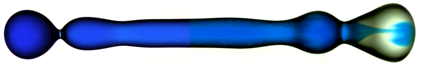
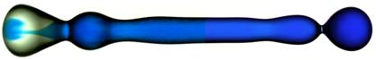
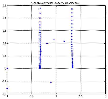
Ploting:
It will plot the spectrum of the operator (complex eigenvalues).
You can view the corresponding eigenvectors by clicking on the desired eigenvalue.
blue is real part, red is imaginary part. Left subplot is the wall-normal velocity and right subplot is the
wall-normal vorticity.
Task:
Find the smallest Reynolds number at which an unstable eigenmode
appears. Which spanwise and streamwise wave number? This eigenmode
corresponds to the Tollmien-Schlichting waves.
Files: osseig.tar.gz
Transient energy growth in channel flow
Description:
This codes is similar to the previous one
to build the dynamic matrix for the OSS operator. It then compute the envelope in time
of the maximum energy growth from initial condition, using singular value decomposition.
Ploting:
It plots the envelope in time of the maximum transient
growth corresponding to the five greatest singular values. By clicking on the growth, you can
view the corresponding initial condition (the one that lead to that energy growth) and
the optimal response (the flow state at the time of maximum growth).
Task:
Check that the highest transient energy growth can be found
for zero streamwise wave number pair, i.e. for streamwise elongated structures,
also known as streaks, or Klebanov modes.
Files: transient.tgz
Boundary layer profile
Description:
This code computes the similarity solution for the boudary layer profile.
It can as well account for a streamwise pressure gradient, and computes the
spanwise profile in the case of Falkner-Skan-Cooke case (flow over a swept wing)
This base profile can then be used for stability analysis, as in the two previous codes.
Ploting:
Plot streamwise and spanwise velocity profile, and their derivatives as a function of the
wall distance.
Task:
At which value of the pressure gradient parameter do we have a zero drag?
Is this adverse or favorable pressure gradient?
Files: fsc.tgz
|