Gallery
You can find here animations illustrating some aspects of my research activity.
To see the movies, you can use Quicktime or VLC. To download the animations to your computer, right click on the movie link ([30M] for instance, indicating the file size in mega-bytes). That way you can see it full screen and in loop.
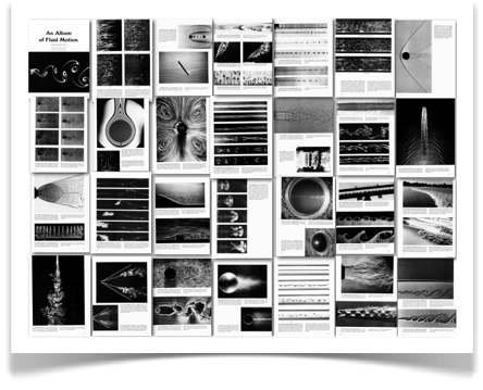
An album of fluid motion
Most of the classical images of fluid motions are gathered in the famous album by Milton Van Dyke. Here is a poster showing the images most relevant to my work. The definition of this file should be enough to print it in A0 format.
Poster:
|
Flapping flag
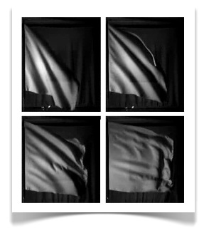
The flag in the wind flaps, and this is an active topic of research to understand how a flow and an elastic body interact and promote instability. Here we show that the flag flaps with oblique waves. We build a simple model for the angle of obliquity based on the structure of the steady state of the flag. The movie below shows the waves observed through numerical simulations of the cloth/fluid using the Navier-Stokes equations, and a wind tunnel experiment using a square of light silk. For more details, have a look at the paper, which we wrote with the aim to have it readable by non-specialists as well...
Animations:
Message de mon grand-père:
Merci pour l'article mais, si je comprends à peu près l'anglais, je ne vois pas à quoi servent ces exercices. Affections. FH
Cher grand-papa,
Il y a pas mal de choses à la fois qui sont présentes dans ce travail. L'instabilité du drapeau est un cas modèle pour les instabilités qui mettent en interaction l'écoulement d'un fluide et le mouvement d'un corps élastique. Des exemples de ce type de phénomènes sont:
1) la manière dont un câble tendu se met à vibrer dans le vent (le sifflement des lignes électrique lorsqu'il fait très froid, ou bien les tuyaux des plates-formes pétrolières, ou bien encore certains pont suspendus),
2) la manière dont le souffle met en vibration les cordes vocales, ou bien la manière dont le souffle met en vibration l'anche d'une clarinette ou d'un saxophone,
3) la nage des poissons est un phénomène analogue, sauf que c'est l'oscillation du poisson qui induit sa vitesse plutôt que la vitesse du poisson qui induit l'oscillation. Ces deux phénomènes ont un lien de "dualité".
Qu'est ce que c'est qu'un "problème modèle?". La manière dont je comprend cela, c'est à la manière d'un territoire et d'une carte. Evidemment le territoire et la carte ne sont pas la même chose. une carte est très différente d'un territoire: c'est un rectangle de papier avec des lignes et des couleurs. Cependant, toutes sortes de gens vont grâce à cette carte pouvoir se faire une idée adéquate de ce à quoi ressemble le territoire, sa structure. La carte c'est comme une vue d'oiseau, utile à nous terriens qui rampons sur le sol. Même si mes lecteurs ne s'intéressent pas exactement au même drapeau que je décrit, ce que j'écrit va pouvoir leur donner des idées, des pistes de recherche, des inspirations...
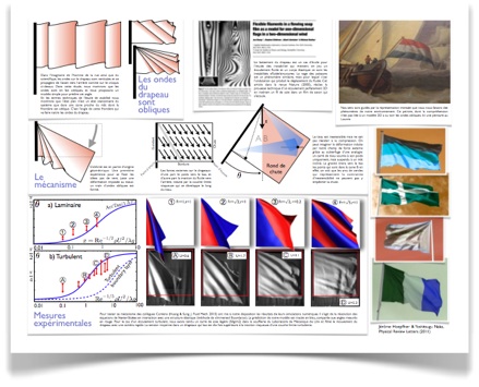
Pas mal de chercheurs ont considéré la manière dont un drapeau se met à battre. Dans l'imaginaire collectif, les ondes du drapeau sont verticales, j'ai fait le test avec les amis et collègues qui se sont intéressés au sujet. Cela signifie qu'ils n'ont jamais véritablement regardé un drapeau, puisqu'il suffit d'en regarder un pour voir que les ondes sont obliques (une fois qu'on le sait...). Cependant, je ne dis pas que tout ce qu'ont fait ces gens est faux... Il ont fait des choses très intéressantes, inspirantes, mais par contre il faut admettre qu'ils ont loupé quelque chose en ce qui concerne les drapeaux que l'on voit battre dans la rue, dans le jardin, devant les mairies, sur les bateaux... Par ailleurs cela illustre un aspect central à la recherche scientifique: il ne suffit pas de voir/regarder les choses pour percevoir l'ensemble de leur comportement; les phénomènes sont multiples et riches et en devenir, et il y a toujours des discours nouveaux à faire entendre pour peu qu'on considère notre environnement d'un point de vue original.
Par rapport à cela, c'est intéressant de voir comment d'autres corps de métiers voient les drapeaux, par exemple les peintres. je suis allé au Louvre pour chercher des drapeaux sur les toiles et j'en ai trouvé avec effectivement des ondes obliques. Depuis des centaines d'années cet angle d'obliquité était là et personne n'y avait fait attention, personne n'avait pensé à les distinguer d'autres drapeaux qui sont dessinés avec des ondes verticales. Voilà, c'est un regard neuf sur un regard très ancien...
Dans cet article je dis d'abord que les ondes sont obliques, ensuite j'explique pourquoi elle le sont. Pour convaincre de ce que j'ai bien identifié la raison pour laquelle les ondes sont obliques, j'ai imaginé un modèle mathématique qui prédit l'angle que font les ondes avec le mât, en simplifiant le problème au maximum, et j'ai comparé cette prédiction théorique avec des mesures expérimentales. Pour ces expériences, nous avons fait flotter des carrés de soie légère dans le flux contrôlé d'une soufflerie. Comme cette prédiction est assez précise, ça peut être considéré comme une preuve, en tout cas c'est convainquant.
Ensuite il y a plusieurs aspects personnels pour lesquels cet article compte pour moi. Premièrement c'est une idée que j'ai eu moi même, et que j'ai pu poursuivre; j'ai réussi à faire vivre cette idée, à la rendre tangible et à convaincre les gens autour de moi. Aussi, c'est un travail que j'ai fait en un temps assez court, et c'est quelque chose de chouette d'arriver à réaliser toutes les étapes de la production d'un article avec cette fluidité, signe de maturation... Aussi, c'est la première fois que je réalise moi-même des mesures expérimentales pour tester mes idées.
Voilà...
Pour faire un article scientifique, il y a tout un tas d'obstacles et besoin d'un grand nombre de savoir-faire. Le professionnalisme c'est la fluidité dans toutes ces étapes. Après cela, il y a la question de la portée de la recherche: est-ce que dans dix ans, dans cent ans on lira encore cet article? Combien de gens sur la planète sont potentiellement concernés par ce propos? Est-ce que cet article va donner envie à d'autres chercheurs de travailler sur ce sujet, les inspirer? Est-ce que cet article fait partie d'un réseau fécond de pensée?
Ou bien alors est-ce que ces quatre feuilles de papier sont stériles et resterons dans l'ombre, oubliées, inutiles? Un gâchis de temps et d'argent...
Est-ce que c'est convainquant?
Voilà, j'espère que tu te portes bien,
J.
Un poster qui représente les différents éléments de cette étude:
The oblique wave on the flag postcard:

|
Optimization for sensitivity analysis
A flow system can show very selective sensitivity to external perturbations like acoustic noise, incomming vortices or eddies. When one instability mechanism dominates, it is easy to predict how the flow will leave its quiet configuration to settle on a turbulent state. When on the other hand several mechanisms are present, or when the mechanisms are complex, a simple stability analysis is not sufficient.
In such cases, it is usefull to analyse the system using optimization. A central question of the sensitivity analysis is "are there perturbations which can grow?", where "grow" usualy is usualy meant in terms of energy, but not necessarily. We can compute the initial perturbation of a time evolution, that lead at a given time T to the maximum possible growth. For this we can use common optimization techniques, for instance here by using the properties of the adjoint system of equations. This system is obtained for the Navier-Stokes equations - that is - the equations that describe the motion of the flow.
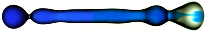
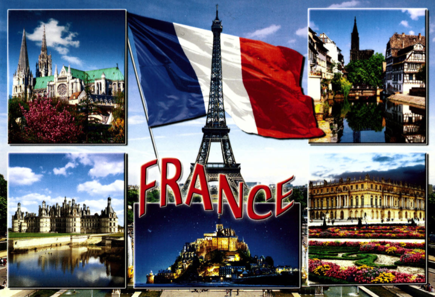
We are here insterested in the sensitivity of a pipe filled with a fluid, that has a localized diameter constriction. This constriction will induce a local acceleration of the flow, and a subsequent strong jet downstream. This jet is surrounded by a recirculation bubble, and shear layers subject to the Kelvin-Helmholtz instability.
In the animations below, you can see the time evolution of the optimization procedure. The two fields are the axial velocity at the top and the radial velocity at the bottom. First the Navier-Stokes system is marched in time until the desired time T for optimization. The chosen initial condition is a random field. The final flow state is used as a starting state for the adjoint equations which are marched backward in time (perturbations advected upstream). The state obtained by marching the adjoint equation is then used as an initial condition for the Navier-Stokes system again, proceding this way for several cycles is some sort of power iteration. Here these iterations converge finally to the initial condition that has the largets energy growth for the target time T.
The animation finishes by marching in time this worst case initial condition, the last image thus represents the perturbation at time T.
Animations:
|
Atomization: two-phase instability
Here are numerical simulations of a two-phase flow made by Daniel Fuster, here at the lab in Paris, using the open-source code Gerris, developped mainly by Stéphane Popinet. I generated the animations out of the data from Daniel.
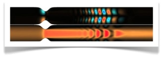
When a liquid jet is in contact with a fast stream of gaz, instabilities lead to the formation of small droplets: a spray. We study these instabilities to predict the drop sizes in different configurations, and understand the mechanisms of formation. A typical application is in combustion: large drops burn too slowly compared to small drops, so its better to have all drops at the same size. Usually the sizes vary widely.
In the animation below, you can see an air/water flow, where the air (light and fast on the top), accelerates the water (heavy and slow) on the bottom, and leads to instabilities and drop formation. The colormap shows the horizontal velocity: red for positive flow and blue for back flow. We then zoom on the injector to see how the interface behaves at the contact betwen the two streams. After that, we visualize the computationnal grid cells, adapting to the interface displacement.
For more on atomization in the lab, see for instance the web pages of Arnaud Antkowiak, Christophe Josseran, Anne Bagué, Stéphane Zaleski.
Animations:
|
Correlated field
Chaos is an inherent feature of many physical system. It is present in flows when instabilities lead to transition to turbulence: growth of small external perturbations lead to an erratic behaviour, dominated by vortices, their breakdown and regeneration. To describe this complex type of behaviour, it is common to consider the statistics of the flow quantities: temporal spectrum at a given spatial location, variance of the flow fluctuation about its mean, two-points correlation... This data tells about the time and temporal scales of the flow field.
Flows are inherently subject to external perturbations: incomming accoustic waves, eddies from other flow processes upstream, structure vibrations...
From the point of view of stability analysis, a flow will be called an amplifier when its behaviour consist in amplifying the incomming perturbations, or an oscillator when its inherent dynamic is so robust that its behaviour is only mildly affected by the external perturbations.
A broad family of amplifiers are the convectively unstable flows: the flow is locally unstable, that is, there exist a process such that perturbations are able to grow in amplitude, but these growing waves are convected away at the same time that they grow. Examples are: Tollmien-Schlichting instability in the boundary layer, Kelvin-Helmholtz instability in the mixing layer with coflowing streams. Here amplifier is synonymous with filter. The own dynamics of the flow will selectively amplify some characteristics of the external perturbations, and damp the rest.
When simulating these flows, it should be worth describing properly the statistics of the incomming perturbations. Indded, flow statistics will be a function of the perturbation statistics.
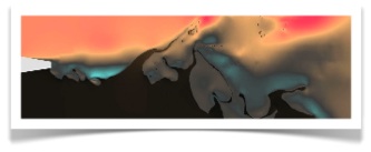
Chaos can be artificially generated by computers. Here it does not emerge from the complex response of a large dynamical system, but from a numerical algorithm. Let us consider a three dimensionnal array of random numbers. This field can be filtered in the three directions (for instance two spatial directions and time) to obtain a correlated field. The filter can be thought as a simple dynamical system, with for instance two degrees of freedom (two states). Due to its dynamics - its eigenvalues - it will let its footprints of the random field: statistics.
In the animation below, you can see this filtered field evolving in time. The parameters of the filter, different in the two spatial directions x and y and in time are changing such as to illustrate different statistical "setpoints". The filters are simply build on two parameters: a decorrelation length: the separation beyond which two points have zero correlation, and the wavelength determining the most energetic oscillation. The two-points correlations in space and time are represented beside the evolving field: on the top the horizontal two-points correlation, on the left side the vertical two-points correlation, and on the top-left corner the two-times correlation.
Animations:
To study the response of complex flows, one can simulate them while introducing these external perturbations, with the correct statistics. The statistics of the response are then extracted from the evolving flow field. An other approach is to solve the equations that governs the statistics itself. This is for instance the aim of the Reynolds-Averaged-Navier-Stokes equation (RANS). For linear systems, as for instance the case of perturbation of low amplitude, the equation for the statistics (two-points correlation) is the Lyapunov equation.
For more on this, see my publication page, and more specifically the paper where we have represented isotropic turbulence as spatially filtered white noise, to study the transition to turbulence in the boundary layer, see stotreaks.pdf.
Artificial turbulence
Here is an other application of these kinds of stochastic techniques, something a bit more technically sophisticated. To simulate turbulent fluid flows, it is very expensive to compute the complete process of transition to turbulence. One way to generate artificial turbulence consist in introducing a large random forcing to excite the flow instabilities, and wait for some time or some space until the turbulence starts to have its natural structure. If the forcing, or the inflow condition is well design, that is is close itself to a "natural" behaviour of the turbulence, then we can get very quickly the good flow properties.
We have developped a method to generate a random field that has precisely the statistics of the turbulence. For this we use as above a filtering technique, but here we use a filter structure known as ARMA: auto-regressive moving-average. This structure is very flexible, and the statistics of the filter output can be very easily fitted to some desired statistics, for instance the statistics of a real turbulent flow. To build this filter, we solve numerically a linear system of equations known as the Yule-Walker equation. This equation is the equivalent of the Lyapunov equation for ARMA filters. Thanks to a recursive solution technique, this equation can be solved very efficiently.
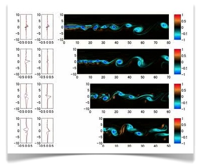
To test this method, we look at a free shear layer. We excite this flow with many vortices at the inflow, and the turbulence is obtained some distance downstream. This simulation is the reference simulation. Then we measure the statistics at three downstream positions, x=10, 20, 30, and then we start three new simulations that have as inflow a synthetic inflow condition: artificial turbulence, which has the same statistics as the reference simulation. This method is described in our paper "Realizing turbulent statistics", see the list of publications.
The animation below shows the vorticity of this testing procedure. The plots on the left show the u, v profile of the reference simulation, and the u, v profile of the artificial turbulence used as inflow. We can see that the flow features are recoverred quickly downstream of the artificial inlets, sign that the artificial turbulence behaves properly.
Animations:
|
Pumping from wall traveling waves
Peristalsis is a mechanism of pumping in tubes, based on the propagation along the tube of a wave of constriction/expantion. It is used for instance to propel and mix the content of the gastro-intestinal tract, see this cite for a very interesting description of the processes of the digestion.
Animations:
Here the flow patterns in a channel with three different wave amplitude of the wall deformation. The pumping is in the direction of the wave.
[3M],
[9M].
Now, instead of a wave of wall deformation, we apply a wave of blowing and suction at the wall. We observe again a pumping effect, but this time, in the direction opposite to the wave.
[3M],
[9M].
|
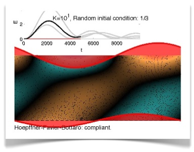
Energy growth in the compliant channel
A compliant surface move in reaction to the flow pressure, like for instance the skin of a dolphin when he swims.
It is believed that under specific surface characteristics this compliance can reduce the flow instabilities, thus postpone the
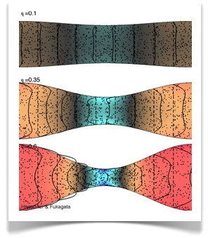
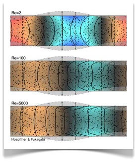
transition to a turbulent flow. If it is so, then the dolphin will feel less flow resistance, swim faster and longer. While in Genova, we started a project on this with Alessandro Bottaro and julien Favier, but instead of looking at instabilities like it is usually done, we compute - using optimization methods - the initial conditions that lead to a large energy growth. It is usefull to compare the obtained growth with the response of the system to random perturbations. For simplicity, we performed the analysis in a channel with two compliant walls.
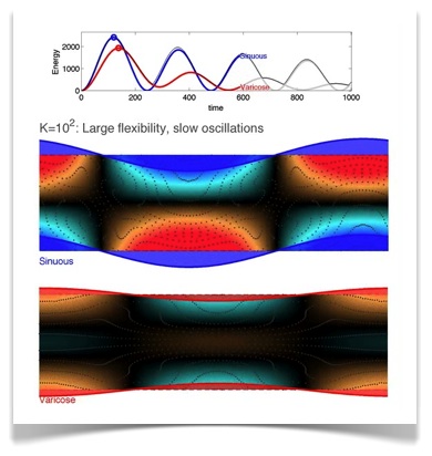
In the animations below, one can see the flow field evolution in time from 3 different random initial conditions, and for three wall stiffness parameters: K from 10 to 100000, that is from rather flexible to rather rigid. We consider flow perturbations that does not vary in the direction of the main stream, thus we can represent the flow in 2D, with a colormap on the streamwise velocity, and the in-plane motion is showed using moving particles. More info in a comming article...
Animations:
Here showing the channel dynamics for several random initial conditions:
[1M],
[9M],
[22M]
Here showing the optimal perturbations, sinuous and varicose:
[3M],
[10M]
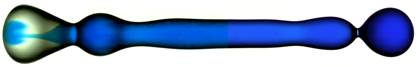
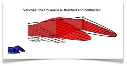
And a sketch of the channel deformation, sinuous and varicose spanwise standing waves:
[1M],
[3M]
|
Optimal control of the Ginzburg-Landau equation
This entry is an illustration of our recent review article on stability and control, applied to the Ginzburg-Landau equation. For more articles on the topic of optimal flow control, see my research page.
Feedback control consist of an coupling an actuator and a sensor to act on a system. The sensor measures some quantity, for instance in a flow the pressure at a given location. This sensor signal is processed and sent to the actuator, which act on the flow, for instance by blowing and suction at a given flow location. Due to this control loop: sensor-to-controller-to-actuator, the controller is able to react to the flow dynamics. Beeing able to react is necessary in cases when the system is exposed to unknown external disturbances.
This is what happens when driving a bicycle. To follow a straight path, it is necessary to constantly adjust the handle direction. Indeed, the system is unstable: if the driver stops controlling, the bicycle and its driver shall fall... The perturbations come from road irregularities, wind and so on. The driver feels when the bicycle is leaning toward one side (sensing), process this information (using his spine) and act to stabilize (turn the handle). The control loop is performed unconsciously, and the law that transforms the sensed signal into an action signal is rather complex. The bicycle dynamics is rather special: to turn left, the handle should be turned first as if to turn right, the center of mass continues straight for a short while, this induces a loss of balance to the left, which is compensated by turning the handle left, with the bicycle turning to the left. This is a example of an inversed response. Two actions must be performed: turn to the opposite direction, wait a little, then turn to the desired direction; the proper timing should be respected.
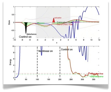
In the animation below, it is the Ginzburg-Landau equation in 1D that is controlled. The dynamics is simple: there is a main convection direction from left to right: external disturbances are convected by the "mean flow". A region of instability is implemented, such that the flow will grow in amplitude while it is convected. Once this region traversed, the system is locally stable again and the amplitude of the flow starts decaying. To this linear convection/diffusion dynamics, one can add some nonlinear effects: a saturation term such that large amplitude variations will be damped, and a "steepening" term, similar to the nonlinear convection term of the Burgers equation. The system dynamics is then composed of: convection to the right by the mean flow, viscous diffusion (that smoothes steep variations), saturation (that damps large amplitudes) and steepening (that generates kinks and high frequency oscillations).
To this dynamics, we introduce a disturbance input, a sensor, an actuator, and an objective output. We build a controller that processes the sensor signal such that the disturbances introduceds are controlled, in order to keep a low objective output amplitude. This controller is optimized for the linearized Ginzburg-Landau equation: the control design (that is building the transfer function from sensor signal to actuation signal) is made without accounting for the nonlinear effects. But finally the controller is applied to the full dynamics.
In the animation below, you can follow the evolution of the uncontrolled state as a response to the disturbance input, both linearized and with the nonlinear terms active. The controller is then turned on, applied to the nonlinear system. The system's energy then decays to its controlled value. The estimator state is presented as well: the controller act as a feedback to the state, but the exact state is not known, it has to be estimated using the sensor information. The energy of the estimation error, which is a measure of the estimation quality is shown. The controller is then turned off, and one can follow the system's state and energy returning to the uncontrolled dynamics.
Animations:
[3M],
[8M],
[30M]
|
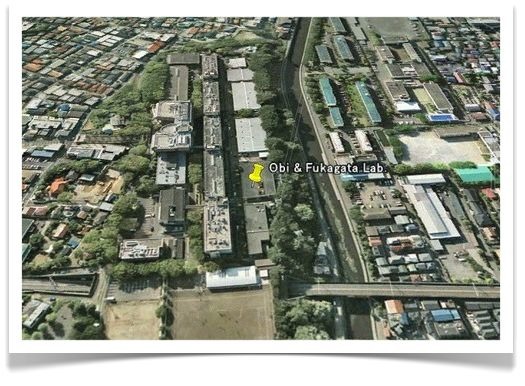
Path to the lab
Here is a visual tutorial on how to reach the Fukagata/Obi lab from Europe. The movie was made by Rio Yokota. A more precise description of the lab location is available here.
Animations:
[7M],
[12M].
|
|